Reading GRAIN Data
Reading and Visualizing GRAIN Data
The GRAIN dataset is distributed as vector geospatial files in both
.parquet and .shp formats.
These files contain the irrigation canal geometries and associated metadata fields such as canal length, slope, use type, country name, and more.
This page provides a quick guide on how to visualize GRAIN canal datasets using
(I) Python and GeoPandas and (II) QGIS.
Both methods are suitable for exploring, styling, and inspecting the irrigation canal networks.
I. Visualizing GRAIN Using Python + GeoPandas
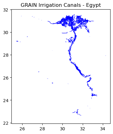
GeoPandas provides a simple Python interface for loading and plotting GRAIN canal files. You may use either the GeoParquet or Shapefile versions of the dataset. Below is an example of viewing the GRAIN canals for Egypt.
GeoPandas provides a simple Python interface for loading and plotting GRAIN canal files. You may use either the GeoParquet or Shapefile versions of the dataset. Below is an example of viewing the GRAIN canals for Egypt.
import geopandas as gpd
import matplotlib.pyplot as plt

# Example file path (modify based on your folder structure)
grain_fp = "./GRAIN_sample_data_EGYPT/sample_outputs/egypt_GRAIN_v1_0.parquet"

# Load the dataset
grain_gdf = gpd.read_parquet(grain_fp)

# Basic info
print(grain_gdf.head())
print(grain_gdf.crs)

#Filter for only Agricultural Canals
grain_irrigation_canals = grain_gdf[grain_gdf["canal_use"] == "Agricultural"]

# Quick visualization
plt.figure(figsize=(8,8))
grain_irrigation_canals.plot(linewidth=0.6, color="blue")
plt.title("GRAIN Irrigation Canals - Egypt")
plt.show()
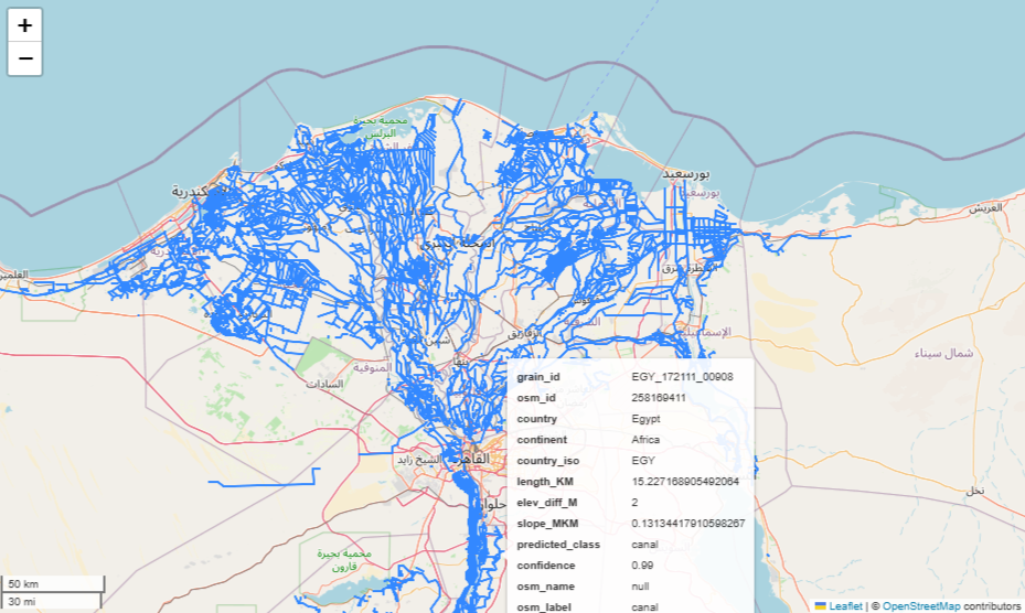
For interactive visualization, the
.explore() method of GeoPandas can be used.
This renders an interactive Leaflet map directly inside a Jupyter notebook, allowing you to zoom, pan, and inspect canal features.
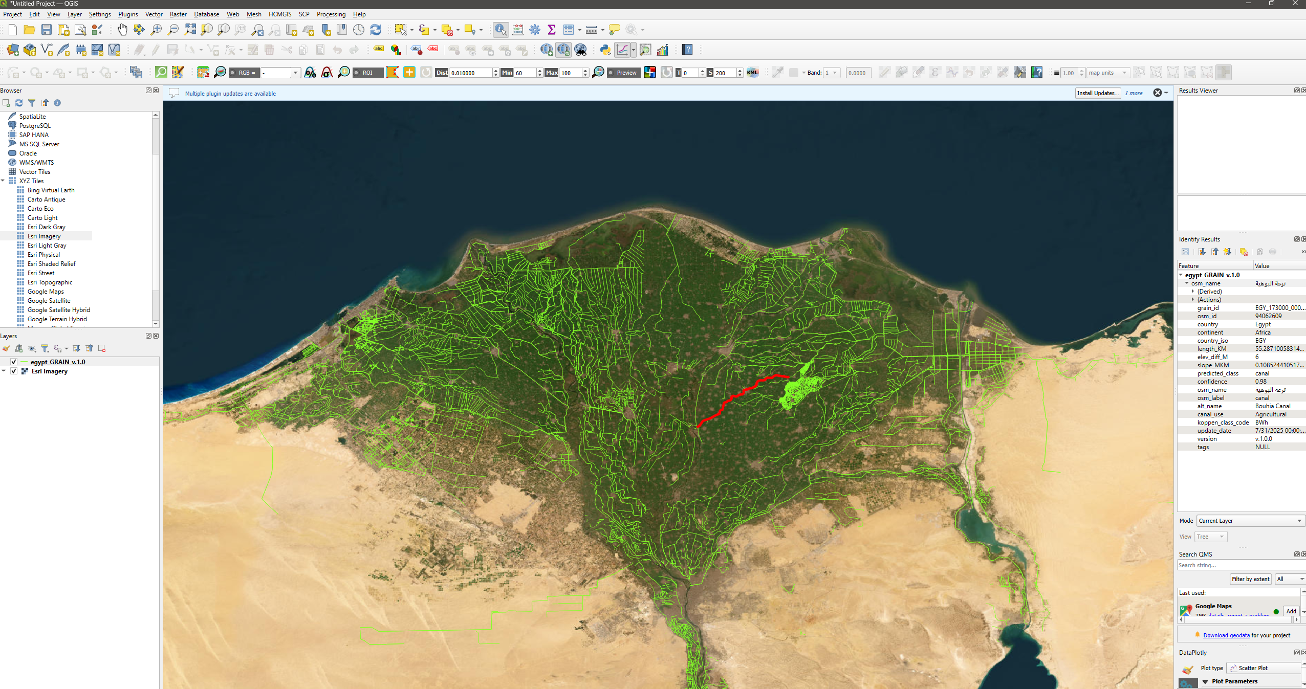
II. Visualizing GRAIN in QGIS
QGIS provides a graphical environment for exploring and styling the GRAIN dataset. Both
.parquet and .shp formats can be loaded directly.
Step 1 — Open QGIS
Create a new empty project.
Step 2 — Load GRAIN data
You can load the dataset using either method:
- Drag-and-drop the
.parquetor.shpfile into the QGIS window - Or use the Browser panel and double-click the file
Step 3 — Style the canals
Right-click the layer → Properties → Symbology.
You may:
- Change line color and thickness
- Use Categorical styling on
canal_use - Use Graduated styling on attributes like
length_KMorslope_mkm
Step 4 — View canal metadata
Open the attribute table to explore fields such as:
grain_id– unique canal identifierlength_KMslope_mkmelev_diff_Mcanal_useconfidence(ML prediction score)koppen_class_code